As an SPSS programmer, you are expected to have a solid knowledge of relational databases, user-friendly software design, and an all-around love for numbers. You will be given a set of requirements to fulfill and must follow those instructions to the letter. In addition, you must have a solid understanding of relational databases and can use SPSS to create and execute queries. You will also be expected to write a program that will allow users to navigate a fixed database.
All these things take time and patience to get good at. AssignU is a platform that connects SPSS experts with students just like you. All you have to do is submit an order and we’ll do the rest!
A sample SPSS assignment
This is an SPSS tutorial dealing with calculating the one-sample T-test within the statistical package for social sciences. If you don’t have the virtual computer lab open already so that you can access another remote desktop and use SPSS, make sure you do that. If you are on campus, you have the luxury of finding a computer lab and getting on a device that has SPSS. So make sure you do that so that you’ll be able to follow along with me as I complete the steps involved in calculating a one-sample T-test. So with that being said, I’m going to proceed with step one listed in your assignment.
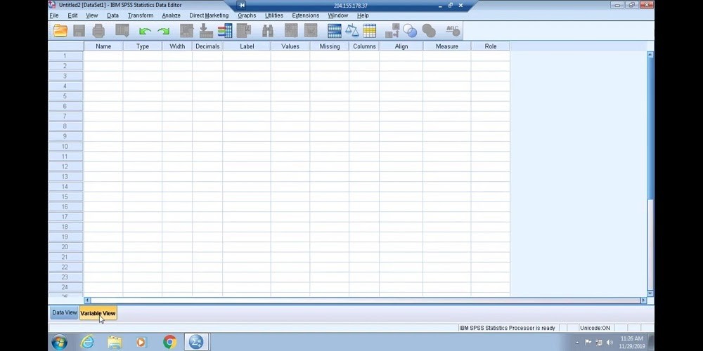
The first step involves you going to a variable view at the bottom of your screen. So right now, you’re in the data view because that tab is glowing. So we’ll toggle over to the variable view. Select it, and you’ll see the variable view become a glow.
You will be creating one variable based on the information in your assignment. Your first row will represent the grade in variable view. All you’ll be inputting into SPSS for this assignment is grades. So each row and SPSS represents a variable. So we will select the first row underneath the name and put in grades.
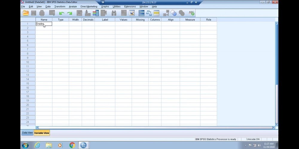
Once we do that, you will see that across the column headers that things are pre-populated.
Now, after you enter the name for your variable, you have the option of selecting a type of variable. There are various types of variables that you can insert into SPSS. We will keep this numeric as shown.
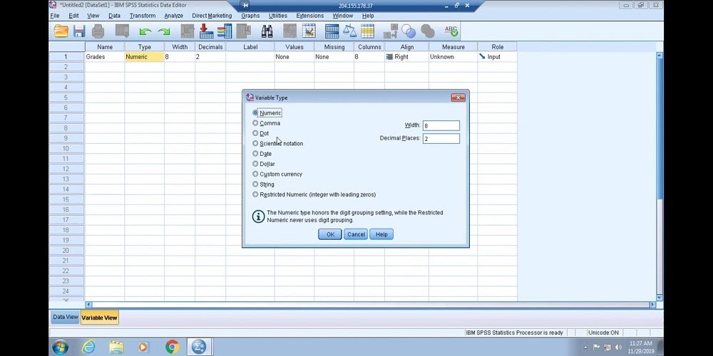
You also have the option of moving forward and expanding the width of your numerical variable. This allows you to dictate how long the numbers, as you will input into the data view, can be. And you’re also able to do that with the decimal places. So we will be entering in digits that have a width of 2, but we don’t necessarily need to make adjustments here. You can’t just leave it as is since having width and decimals that are far and above what you need is okay, and you want to air on the side to make sure that the width isn’t too small. Now, going over to labels, you can add in an extended name for your variables as shown (See Final Grades)

This extended name will show up when you calculate your one-sample T-test. In other words, it’ll show up in the output.
You can assign labels associated with specific numbers for values, if you need to, for your variable. If you have nominal or ordinal or maybe internal data in some instances, you should be doing this. Otherwise, you’re going to bypass it. We have a variable that is very much ratio starts from zero, that zero indicates an absence of the variable. Ratio variables have all the defining characteristics of nominal ordinal and interval variables. So we don’t necessarily need to go to values to assign labels to certain numerics along with the significant intervals.
Missing is a header that you will utilize if you have some missing numerics in your data set. That does not apply to this assignment, so don’t even worry about that. You can keep the columns at eight and go with the correct alignment.
In terms of measure, make sure you’re working with the ratio variable you select scale. Scale involves interval and ratio data. So you’ll want to make sure you select that. Once you do all of that, you have efficiently set up your variable, toggle back over to dad of you, and now you’ll see grades at the top of the column header for one variable and notice how everything else says var, var, var.
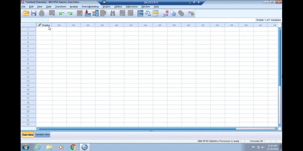
These “var” are instances of variables that haven’t been set up that don’t necessarily apply to your study. But these will change if you were to set up additional variables beyond grades. From here, which you need to do is insert your data. So going to your SPSS assignment, you’ll insert all of your grades as shown.
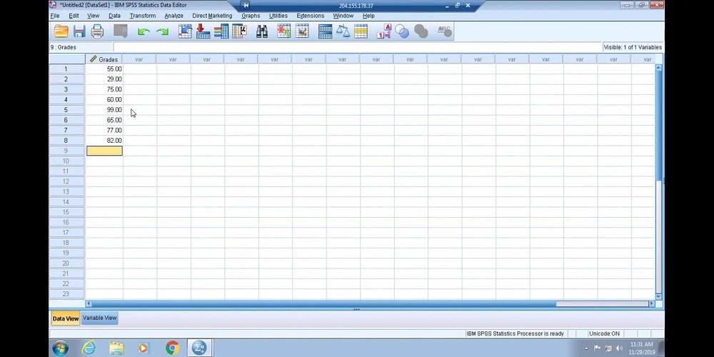
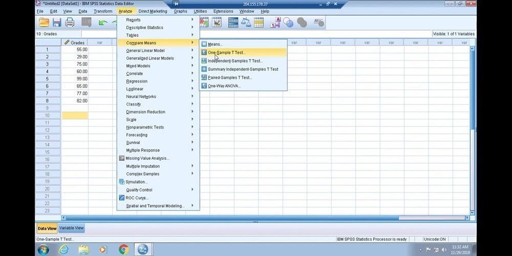
So grades are inserted into the data review part of SPSS. Please keep in mind for my students that I would add two of these grades. So make sure that you’re not just doing step by step what I’m doing, but that you’re relying on your assignment to be the guide for the data that you enter. From here to calculate the one-sample T-test. You will click analyze on the toolbar, and then you’ll scroll down to compare means. And then from compare means you will go to one-sample T-test.
Now, what you do here is you take the highlighted column label for the set of scores, which is grade, and you will move that over into the test variable box. Based on the information in your assignment, what you will do, and then the test value box at the bottom of the one-sample T-test window, is entered the hypothesized value for the mean from the null hypothesis. In this particular case, it is 75. So 75 is the population parameter that you’re given or the population mean. Then these final grades consist of the sample, and ultimately a sample mean will be calculated from it that will be compared to the population made up of 75. From there, you click, okay. And once you click, okay, it will give your data output screen.
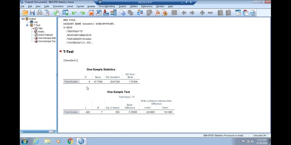
You see a one sample statistics descriptive table laid out for you, letting you know that you had eight individuals in your sample. On average, the grades were 67.75, the standard deviation was 20 points, And the standard error of the mean is 7.38 if you round.
If you come down to the actual one sample T-test, the T that you would end up with if you did 67.75 minus 75 over the standard error of the mean, you would end up with -.982. The degree of freedom would be 7. And it is not significant because this alpha level was not .05 or below. That’s important to note when you’re trying to figure out if the one-sample T-test is substantial or not. If in the sig (2-tailed) column you don’t see a decimal that’s below .05, then you know it’s not significant. That’s important to keep in mind. So we got an insignificant T-test. In other words, 67.75 is not significantly different from 75, probably because, as you can see, the variation is relatively large.
The main difference essentially is if we took 75 from 67.75, you would have 7.25, and then it gives you confidence intervals based on the statistic that was calculated.